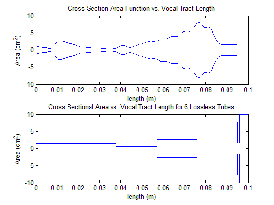
| Part A of this project deals with the synthesis of an assigned English vowel sound using a series of concatenated tubes to approximate the shape and characteristics of the human vocal tract so that discrete time signal processing techniques can be applicable. This web page will explore only the /o/ sound as produced by a child but other synthesized vowel sounds will be provided for the sake of comparison. Part B then deals with linear prediction to re-synthesize speech using Levinson's recursion technique. The software package MATLAB was used for all algorithm implementations; links to the source code are provided in each part. Unless otherwise noted, the sampling rate for this study is 8kHz thus making the bandwidth of the produced speech 4kHz. Part A 1. To generate a continuous cross sectional area function, A(x), from the provided area vector MATLAB's spline function is used to "upsample" using cubic spline techniques. This function can be seen in the top plot in the figure below. The bottom plot of this figure illustrates the area values for N tubes with N being the number of tubes calculated based on l (the length of the vocal tract), Tau (a constant based on the signal's bandwidth) and c (the speed of sound in air). To calculate the length of the vocal tract (l) .05 (the length of each segment in cm) is multiplied by the length of the vowel vector and since a child has a vocal tract that is half the length of an adult male this value is then multiplied by .5. For a child /o/, N was calculated be equal to 6. The bottom plot of the figure below shows an extra, fictitious tube to represent the 'outside world' that does not reflect. In the top plot the fictitious tube is shown by the emptiness at the that the end of the vocal tract is open to.
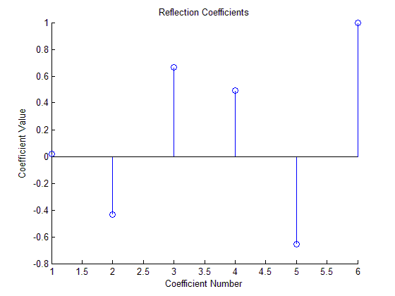
Based on the six areas shown in the bottom plot of the figure above five reflection coefficients are calculated. The fictitious tube is assumed to have a reflection coefficient of 1 in a lossless setting and is accounted for in the sixth reflection coefficient. Shown below is a stem plot of the reflection coefficients.
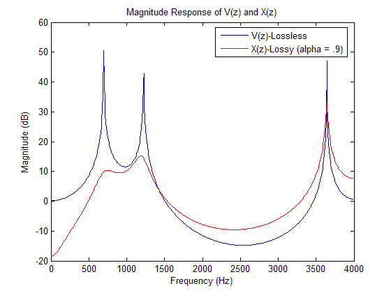
2. Using the reflection coefficients calculated above the denominator coefficients for the transfer function V(z) = UL(z)/UG(z) are calculated. This transfer function mathematically models how the vocal tract discussed and shown previously 'colors' the sound traveling through it. It is responsible for the timbre of human voice. The resonances it possesses are known as formants and can be seen in the plot shown after the discussion of part three. Since this transfer function is lossless its numerator is simply Az-N/2 with A being equal to 1. 3. Representing the vocal tract as a lossless medium will result in a transfer function that has formants of infinite amplitude and zero bandwidth. This is not accurate and does not lend itself to a proper way to synthesize vowel sounds. While it is impossible to account for all losses of the vocal tract using discrete time procedures accounting for the approximate loss due to radiation is relatively simple. To do this the numerator of the transfer function calculated in part 2 is multiplied by 1-αz-1. A new transfer function A(z) is then created. The resulting transfer function's formants now have finite bandwidths and do not 'blow up' to infinity. Both the lossless and the lossy spectral envelopes that result from their respective transfer functions are show below.
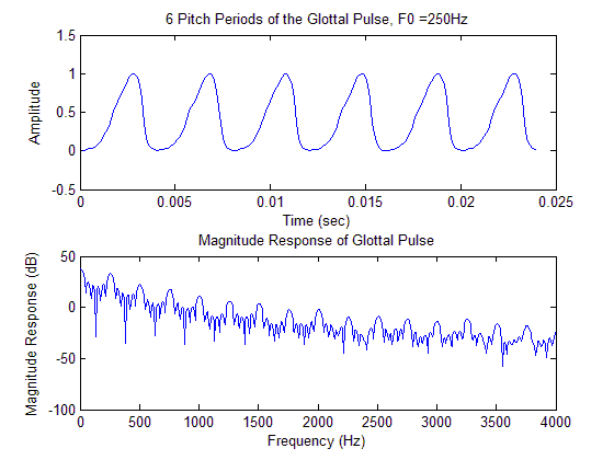
4. The next step in producing a vowel sound is simulating the glottal pulse that is produced by the vocal folds during voiced sounds. The vibration of the vocal folds is what is responsible for the pitch of human voice. The first step to modeling this is to convolve B-nu[-n] (.85 was used for B) with itself. Only doing this does not produce an entire cycle of a glottal pulse so the end of the result of the convolution had to be extended gradually to zero to model the glottal pulse as accurately as possible. Also, to increase accuracy, a slight amount of noise was added to the glottal pulse. The spline function was then used to make the length of the glottal pulse as long as it had to be to obtain the desired pitch frequency. In the case of a child a reasonable pitch frequency is understood to be 250Hz. Six pitch periods of the glottal pulse that was created using the aforementioned method is shown in the figure below along with its magnitude spectrum. The pitch frequency can be observed in the magnitude spectrum plot by calculating the distance between each large 'lobe' on the graph. It may be easier to notice that there are four equally spaced large lobes every 1000Hz thus yielding a distance between them of 250Hz.
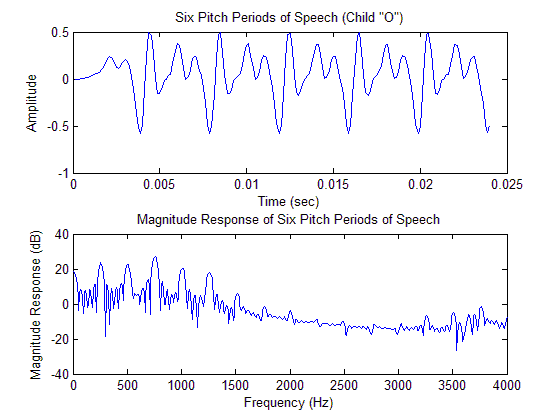
5. Finally, to generate six pitch periods of speech the glottal pulse is filtered with the lossy transfer function X(z) using the MATLAB filter function. The waveform and magnitude spectrum plots for the six pitch periods of speech are shown below. Notice that the glottal pulse is responsible for the periodicity of the signal while X(z) is responsible for shaping the spectral envelope of the magnitude spectrum.
6. Since six pitch periods of a 250Hz sound is only audible as a 'click' two seconds worth of glottal pulses are created and filtered with X(z) to generate two seconds of 'speech.' Click here to listen to the child /o/ that was generated by this algorithm. Below are links to other vowel sounds produced by this algorithm. Though not exactly required they are provided for comparison purposes.
Male /o/
Female /o/ Summary: The vowels created in this
part do not exactly sound natural but it is possible to distinguish
between /o/ and /e/ so in that sense they are correct. Since
actual human vowel sounds are quasi-periodic the ones created here
will sound more robotic than normal human speech. Part B 1. MATLAB code was written to implement the recursive Levinson recursion algorithm and can be found here along with the code for steps 2-4 of this section. 2. One signal frame (25ms in length) of the child /o/ sound generated in the previous part is selected and used as input to the Levinson recursion algorithm in (1). Before being inputted into algorithm the signal frame is sent through a pre-emphasis filter and windowed with a hanning window. The pre-emphasis filter is a high pass filter that is necessary because the energy in human speech decreases as frequency increases. The pre-emphasis filter boosts high frequencies and attenuates low frequencies in an attempt to flatten out the spectrum. The order for prediction in this part was selected to be 6 to match the number of tubes that were calculated and used in Part A. This will allow for an exact comparison. The linear prediction and PARCOR coefficients that are outputted by the Levinson recursion algorithm for this particular input are listed in the table below. The linear prediction coefficients are listed as they are in the denominator of the transfer function, that is they are preceded by a 1 and negated since the denominator equation is 1-Σαkz-k with the sum going from k=1 to p and α representing each the linear prediction coefficient.
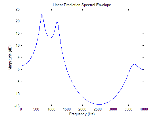
3. The linear prediction spectral envelope produced by the linear prediction algorithm discussed above is shown below. The three formants are almost in the exact same locations as they were in Part A but the magnitudes are greater. This could be due to the gain factor that was used or the coefficients used in the pre-emphasis filter . Both of these values were experimented with but to no avail. The plot shown below uses both of the given equations for pre-emphasis and gain and, when compared to all of the other plots arising from 'experimental' methods that were tried, it is the most correct.
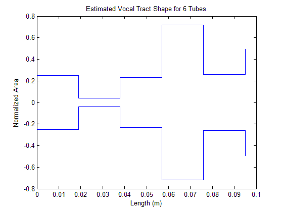
4. From the coefficients determined in (3) the shape of the vocal tract shape can be estimated. It is shown below. The shape is similar to the actual shape plotted in part one but the proportions are a bit off. The general shape goes from wide to narrow to wide to wider and then back narrow which is the same pattern that the shape in Part A follows.
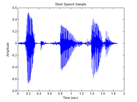
5. In this part a short speech sample was created using three words that were recorded in project I. The short phrase is simply "vote for father" and can be heard by clicking the link in the previous sentence. The sampling rate of file is 16kHz, as specified in the project description. Its time domain waveform is shown below.
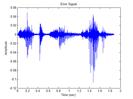
6, 7 & 8. Using short-time analysis the utterance provided in (5) is windowed using a 20ms Hamming window with an overlap of 50% and then put through a linear prediction algorithm with an order of 20. The steps included in the first half of the linear prediction operation (in order) include: windowing the signal, performing autocorrelation on the windowed signal, putting the windowed signal through a pre-emphasis filter to boost the high frequencies, storing the coefficients used in the pre-emphasis filter, performing autocorrelation on the pre-emphasized signal, putting the pre-emphasized signal through the Levinson algorithm implemented in (1), inverse filtering the signal using the coefficients generated by the Levinson algorithm and then storing the coefficients used in the inverse filtering signal. After this process is performed on every frame overlapping and adding of the output frames to obtain the error signal e(n). The wav file of the error signal is provided here and its plot is shown below.
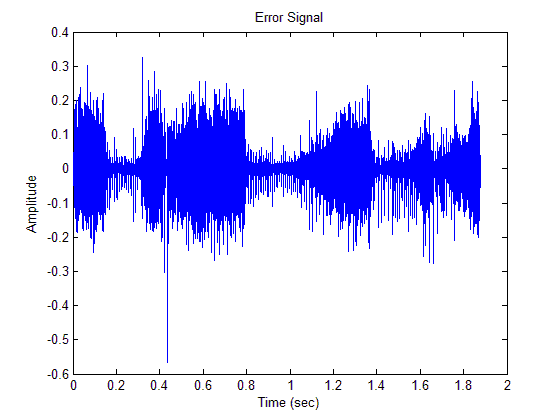
After realizing that the gain computation of the inverse filter was omitted from the above process a new error signal was obtained when including the gain. Audibly it sounds worse than the previous error and has greater amplitude but it results in a better sounding output in (9). The wav file of the error with the gain computation included can be heard here and the plot is shown below.
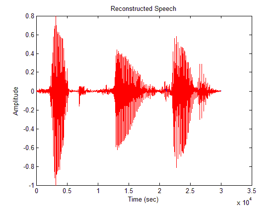
9. Using all of the stored coefficients and the error signal generated without the gain factored in from (8) the original speech signal s(n) is reconstructed. In theory this should be exact reconstruction but somewhere in the process the amplitudes of a some samples are increased. Perceptually the original signal and the reconstructed signal are nearly identical but their residues are not all zeros like they should be. The cause of this amplification was investigated thoroughly but the cause was not found and still remains unknown. The wav file of the reconstructed speech can be heard here and the plot of it is shown below.
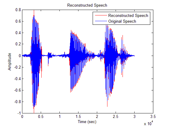
When the gain factor is included in the process the reconstructed speech is not much different but the amplitudes are a bit closer to the original. The reconstructed speech with the gain factor included can be heard here and a plot of it is shown below. The plot shows both the original file and the reconstructed file on the same plot, in different colors, for an easy comparison. The MATLAB source code for sections 5-9 can be downloaded here.
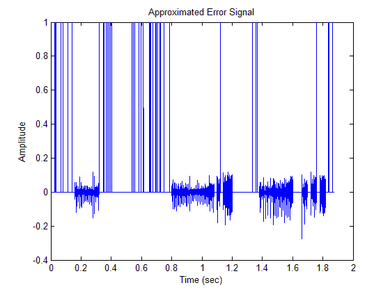
10. The last section of this project deals with a very crude compression implementation using the output from the previous sections. To achieve compression the error signal from (8) (with the gain included) is approximated by either a series of impulses for voiced sections or noise for non-voiced sections. To do this the error signal is examined on a frame by frame basis using a frame size of 20ms. Each frame is determined to be either voiced or unvoiced. If the frame is unvoiced it is left unaltered. If the frame is voiced then every sample above a certain threshold is set equal to one and every sample below that value is set to zero. This process half wave rectifies voiced frames when modeling them as a series of impulses. The most effective threshold was found to be .12 and that's what is used here. A less heuristic method of determining which frames are voiced and unvoiced would be to calculate the spectral flatness measure and base the decision off of that since noise-like signals have relatively flat spectra. The MPEG-7 standard outlines the calculation of spectral flatness but the implementation of it here is beyond the scope of this project. The altered error signal is shown below and can be heard here.
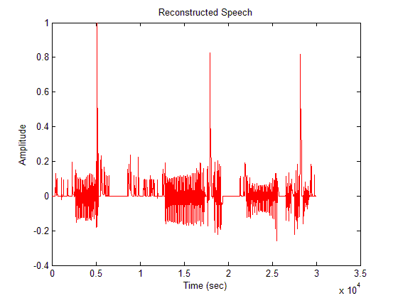
This error signal is then put through the same reconstruction algorithm that was used in (9). The output of this can be heard here and the plot is shown below. The MATLAB code for this last part is available here.
From the above plot it is obvious that voiced sections remain half wave rectified and that there is a bit of clipping. The gain for each frame of the transfer function would have to be altered to fix this. Even though the error signal is altered this speech is still intelligible but there is a fair amount of clipping in the signal which is never pleasant to listen to. It is obvious that this method could be tweaked to increase quality and offer a decent amount of compression.
|
|||||||||||||||||||||||||||